 Figure 1: Heatmap of 1.3 billion taxi rides taken in New York City
 (Data provided by the NYC Taxi & Limousine Commission)[/caption] When you’re ready to render all of the data you’ve collected, you will run into another common choke point. If you are trying to visualize millions or billions of data points you will be putting a massive load on your rendering engine and you are going to be waiting a long, long time. GeoWave solves this by effective use of spatial subsampling. Each pixel on a map can only represent a finite amount of data, so GeoWave transforms the pixel space on the map using the underlying datastore to restrict the amount of data rendered onto a single pixel. In the example below, we are using this spatial subsampling to display 52 million GDELT data points. In the world of Big Data this is a relatively small amount of data, but it would still be more than enough to cause headaches for any analyst while he or she waits hours to view the data. Using GeoWave to help visualize data turns this into a process that takes a second. The subsampling is then performed again as you zoom in so that the best possible visualization of the data is maintained. [caption id="attachment_5218" align="aligncenter" width="1210"]
 Figure 2: 52 million GDELT data points mapped in seconds using GeoWave subsampling[/caption]
[caption id="attachment_5219" align="aligncenter" width="1207"]
Figure 2: 52 million GDELT data points mapped in seconds using GeoWave subsampling[/caption]
[caption id="attachment_5219" align="aligncenter" width="1207"]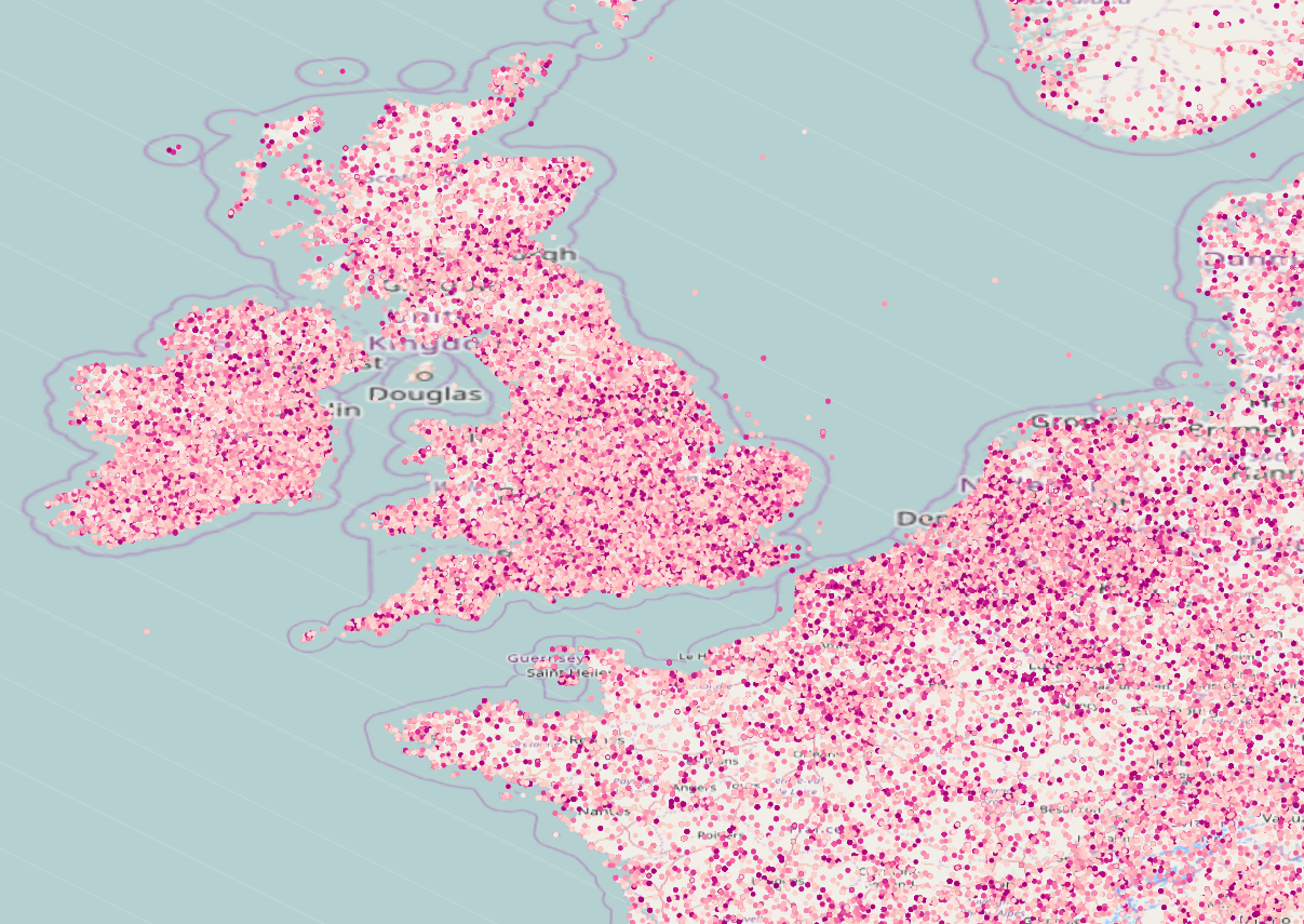 Figure 3: The subsampling is re-performed as the zoom level is changed[/caption]
GeoWave also offers a suite of functionality to help you analyze your dataset, and we do truly mean “your data.” We released GeoWave version 0.9.3 in December with full HBase support, initial Bigtable support and major renovations to our documentation, including a Quickstart Guide for new users. As our customers’ needs continue to grow and change over time we continue to add features and functionality to GeoWave. We look forward to adding support for additional datastores, advancing our analytics, and further usability enhancements in the near future.
GeoWave is currently packaged with ingest formats for many common geospatial data types, and any other data type can be easily added as a plugin. GeoWave is packaged with a set of statistics such as: ranges over an attribute, cardinality of the number of stored items, histograms over the range of values, and much more. Available analytics include kernel density estimation (as seen in Figure 1), nearest neighbors and KMeans analysis using multiple clustering methods. Look for examples of some of these analytics in future GeoWave blog posts.
Figure 3: The subsampling is re-performed as the zoom level is changed[/caption]
GeoWave also offers a suite of functionality to help you analyze your dataset, and we do truly mean “your data.” We released GeoWave version 0.9.3 in December with full HBase support, initial Bigtable support and major renovations to our documentation, including a Quickstart Guide for new users. As our customers’ needs continue to grow and change over time we continue to add features and functionality to GeoWave. We look forward to adding support for additional datastores, advancing our analytics, and further usability enhancements in the near future.
GeoWave is currently packaged with ingest formats for many common geospatial data types, and any other data type can be easily added as a plugin. GeoWave is packaged with a set of statistics such as: ranges over an attribute, cardinality of the number of stored items, histograms over the range of values, and much more. Available analytics include kernel density estimation (as seen in Figure 1), nearest neighbors and KMeans analysis using multiple clustering methods. Look for examples of some of these analytics in future GeoWave blog posts.